Multi region hearter tutorial
1. Analysis overview
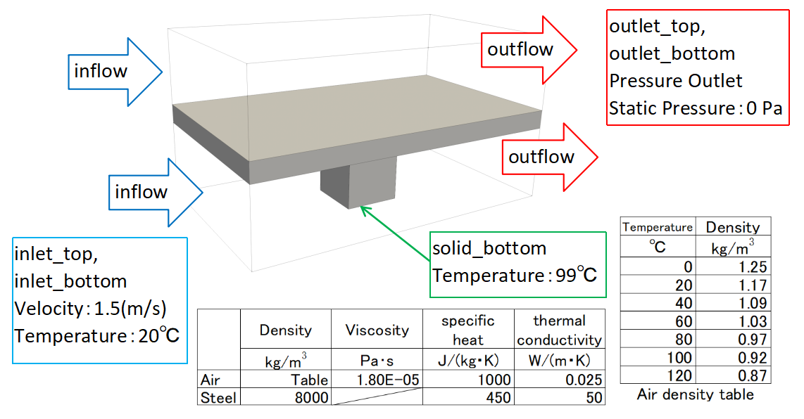
This analysis observes the fluid flow and temperature distribution around a structure whose lower part generates heat.
This is an analysis where there is a steel wall of 10 mm thickness connected to a square pillar of 15 mm per side and 40 mm in height made of steel, and air flows at 20°C through the space above and below the wall.
The underside of the column is set to 99°C to check the temperature distribution in the wall, column, etc.
Physical properties of air and steel are approximated.
The density of air is a function of temperature dependence in tabular form.
The relationship between density and temperature is shown in the figure on the right.
Set the viscosity of air to 1.8 x 10⁻⁵ (Pa-s), the specific heat to 1000 J/(kg-K), and the thermal conductivity to 0.025 W/(m-K).
Set the density of iron to 8000 (kg/m3), specific heat to 450 J/(kg-K), and thermal conductivity to 50 W/(m-K).
Download the geometry data used for this analysis here.
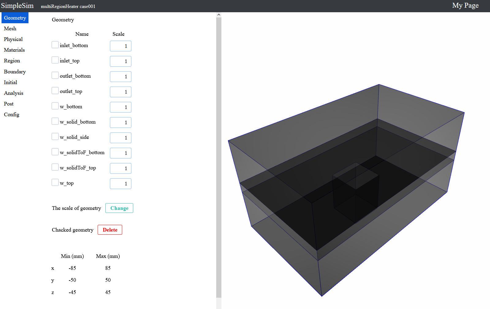
2. Geometry
When you access the case file, you will see a screen like this.
Update the shape file for analysis on this screen.
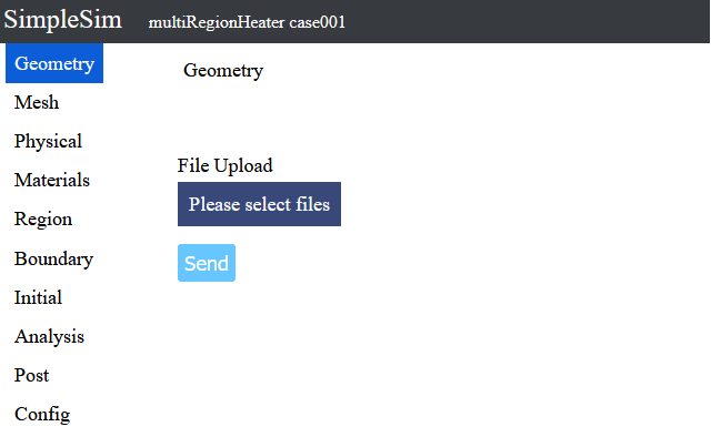
When you unzip the file that can be downloaded in "1. Contents of analysis", there is "multiRegionHeater.stl" inside, so this time we will use it.
Press the "Choose File" button, select "multiRegionHeater.stl" and press the Open button.
"multiRegionHeater.stl" will be displayed under the "Select a file" button, so press the send button to upload the file.
When the upload is complete, the 3D model will appear on the right side.
Drag the left button to rotate the 3D model.
Drag the center button or rotate the center wheel to zoom in or out on the 3D model.
Drag the right button to translate the 3D model.
The buttons [+x][-x][+y][-y][+z][-z] direct the viewer in the direction indicated on the button.
The buttons [+90deg↷][-90deg↶] rotate the line of sight 90° clockwise and counterclockwise.
The buttons [+axis] and [-axis] show or hide the axis.
[Switch Camera] button changes the perspective projection/parallel projection.
[Fit Camera] button fits the 3D model to the size of the screen.
3. Mesh
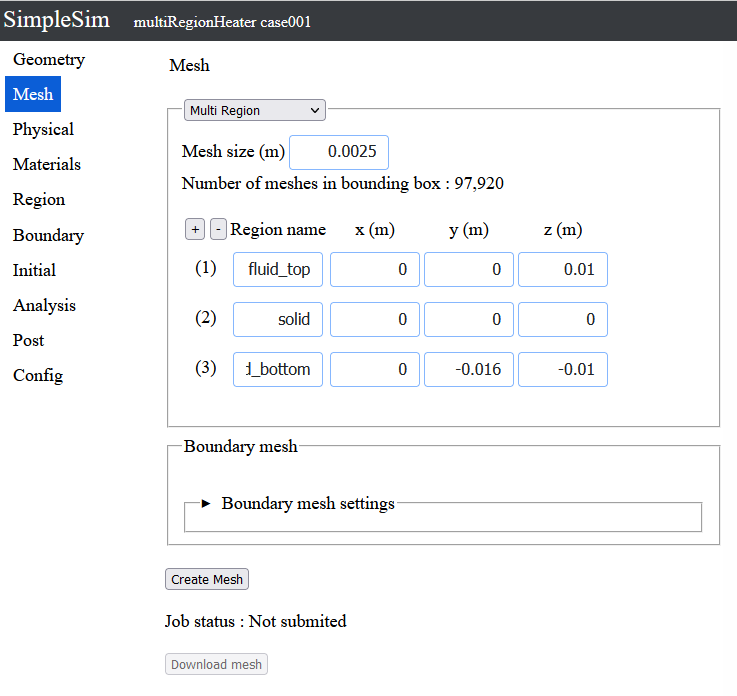
By pressing the mesh button on the left, you can move to the mesh settings screen.
Change the mesh type to "multi-region".
Enter "0.0025" for the mesh size.
Increase the number of regions to 3 by pressing the [+] button to the left of the region name.
Enter "fluid_top" for the region name in (1).
Enter (0, 0, 0.01) in position (1)
Enter "solid" in the region name at position (2)
Enter (0, 0, 0) in position (2)
Enter "fluid_bottom" for the region name in (3).
Enter (0, -0.016, -0.01) at position (3)
Now that the mesh input is complete, press the Create Mesh button and a confirmation window will appear, press "Yes" to create the mesh.
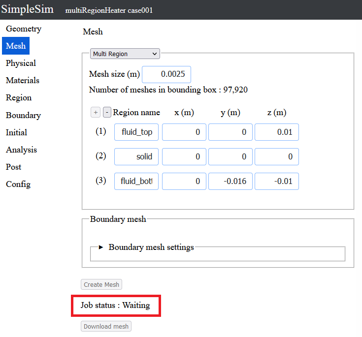
The job has been submitted and the job status is waiting for its turn.
When it is your turn, mesh creation will begin.
You can wait for the mesh to be completed, but you can proceed with the analysis settings without waiting for the mesh to be completed.
*If you wait until completion, you can download the mesh.
4. Physical models
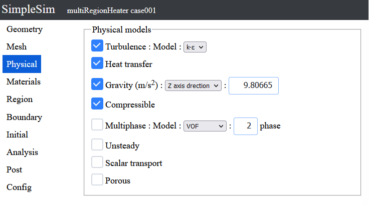
By clicking the Analysis Conditions button on the left, you can move to the Analysis Conditions setting screen.
In this screen, you can turn on/off heat, gravity, etc.
Turn on turbulence, heat transfer, gravity, and compressible.
Change the direction of gravity to "z-axis direction".
5. Materials
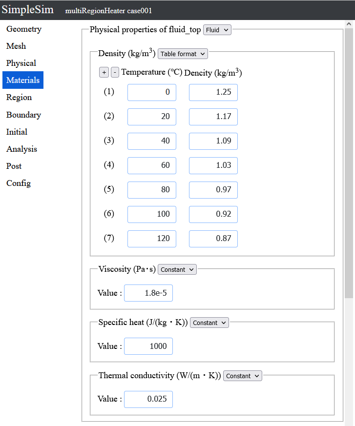
Clicking on the left side of the "Physical Property Values" button will take you to the "Physical Property Values" screen.
Set from the physical property values of fluid_top.
Change the density to a tabular format.
Press the [+] button to the left of temperature 5 times to allow 7 inputs.
Enter "0" for temperature (1).
Enter "1.25" for the density of (1).
Enter "20" for the temperature in (2).
Enter "1.17" for the density in (2).
Enter "40" for temperature in (3).
Enter "1.09" for the density in (3).
Enter "60" for temperature in (4).
Enter "1.03" for the density in (4).
Enter "80" for temperature in (5).
Enter "0.97" for the density in (5).
Enter "100" for the temperature in (6).
Enter "0.92" for the density in (6).
Enter "120" for the temperature in (7).
Enter "0.87" for the density in (7).
Enter "1.8e-5" for the viscosity.
Enter "1000" for specific heat.
Enter "0.025" for thermal conductivity.
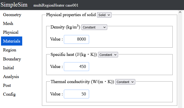
Change the physical property value of solid. Change the select box to the right of the solid physical property value to "solid region".
Enter "8000" for Density.
Enter "450" for Specific Heat.
Enter "50" for Thermal Conductivity.
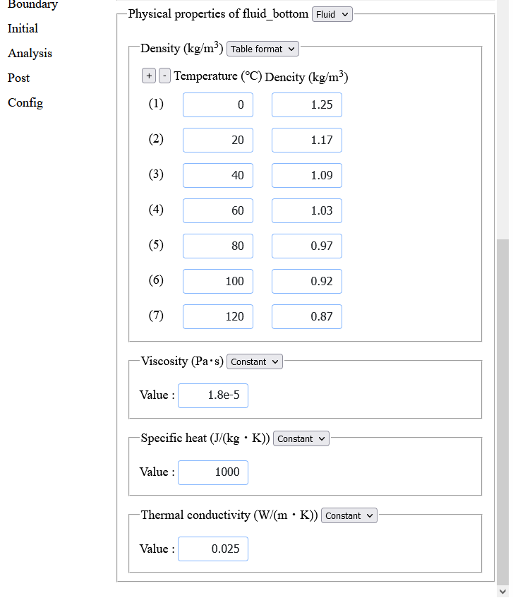
Change the physical properties of fluid_bottom. Change the density to tabular form.
Press the [+] button to the left of temperature 5 times to allow 7 entries.
Enter "0" for temperature (1).
Enter "1.25" for the density of (1).
Enter "20" for the temperature in (2).
Enter "1.17" for the density in (2).
Enter "40" for temperature in (3).
Enter "1.09" for the density in (3).
Enter "60" for temperature in (4).
Enter "1.03" for the density in (4).
Enter "80" for temperature in (5).
Enter "0.97" for the density in (5).
Enter "100" for the temperature in (6).
Enter "0.92" for the density in (6).
Enter "120" for the temperature in (7).
Enter "0.87" for the density in (7).
Enter "1.8e-5" for the viscosity.
Enter "1000" for specific heat.
Enter "0.025" for thermal conductivity.
6. Regions
By clicking the Boundary Conditions button on the left, you can move to the Boundary Conditions setting screen.
There are no items that can be changed in the area settings at this time.
7. Boundary conditions
By clicking the Boundary Conditions button on the left, you can move to the Boundary Conditions setting screen.
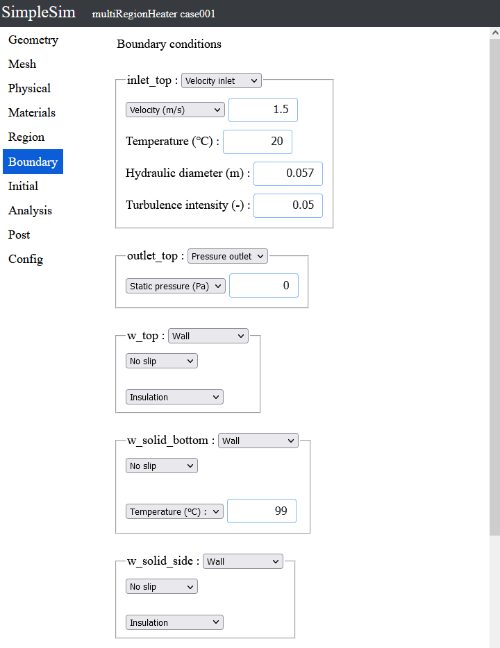
Select a velocity boundary from the select box to the right of inlet_top.
A velocity boundary is a boundary where the flow enters at a constant velocity perpendicular to the boundary.
Enter "1.5" for velocity.
Use the default value of "20" for the temperature.
Enter "0.01" for Hydraulic Diameter.
Use the default value "0.05" for turbulence intensity.
Select the pressure outlet boundary from the select box to the right of outlet_top.
The pressure outlet boundary specifies the pressure value on the boundary.
Use the default value "0" for pressure.
Select the wall surface from the select box to the right of solid_bottom.
Select "Temperature (°C)" from the select box that is insulated.
Type "20" in the text box to the right of it.
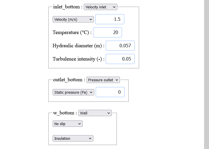
Select a velocity boundary from the select box to the right of inlet_bottom.
A velocity boundary is a boundary where the flow enters at a constant velocity perpendicular to the boundary.
Enter "1.5" for velocity.
Use the default value of "20" for the temperature.
Enter "0.01" for Hydraulic Diameter.
Use the default value "0.05" for turbulence intensity.
Select the pressure outlet boundary from the select box to the right of outlet_bottom.
Pressure uses the default value of 0.
Leave the other boundaries at their default values of wall, no scour, and adiabatic.
8. Initial conditions
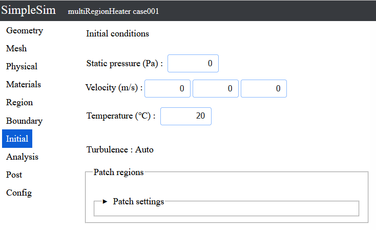
By pressing the Initial Conditions button on the left, you can move to the Initial Conditions setting screen.
All default values are used.
9. Analysis
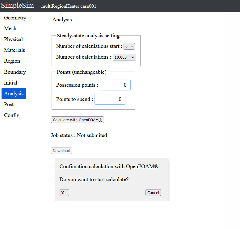
By clicking the Analysis button on the left, you can move to the Analysis Setup screen.
The calculation will be performed 10000 times without convergence judgment.
When you press the "Calculate with OpenFOAM" button, a window will appear asking "Do you want to start the calculation?" and press "Yes" to start the analysis.
10. Post processnig
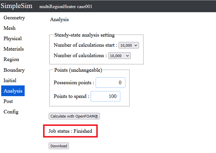
When the calculation is complete, the analysis data can be downloaded.
Click the "Download" button to download the data.
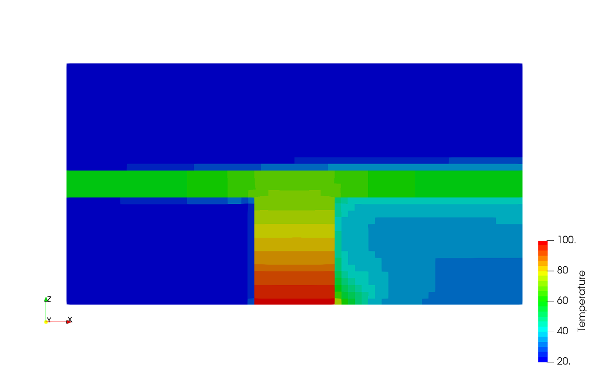
Please unzip the downloaded file and post-process it with ParaView or other software.
The temperature distribution in the center cross section will look like this.
To the Tutorial List
Update June 04, 2023